Understanding your cat's meows using a neural network
“Meow” — I’m sorry? “Meow!” — Oh, right! Here you go.
What if I could understand exactly what my cat is trying to tell me? We live in 2021, which is basically the future. How hard can it be?
What’s on your mind, little Loki? With the power of neural networks, maybe soon I’ll know.
A dataset of meows
A group of dedi_cat_ed researchers from northern Italy has recently released a public dataset of cat vocalizations (let’s call them “meows”). 21 cats from two different breeds were exposed to three different situations while a microphone was listening:
- Brushing: The owner brushed the cat in a familiar environment.
- Isolation: The cat was placed in an unfamiliar environment for a few minutes.
- Food: The cat was waiting for food.
In total, the dataset comprises 440 audio files.
Dataset statistics
The dataset is not evenly split between those three situations.
Number of recordings per situation:
Neither is it evenly split between cat breeds or the sex of the cat. The figure shows number of recordings per breed:
Number of recordings per sex of the cat:
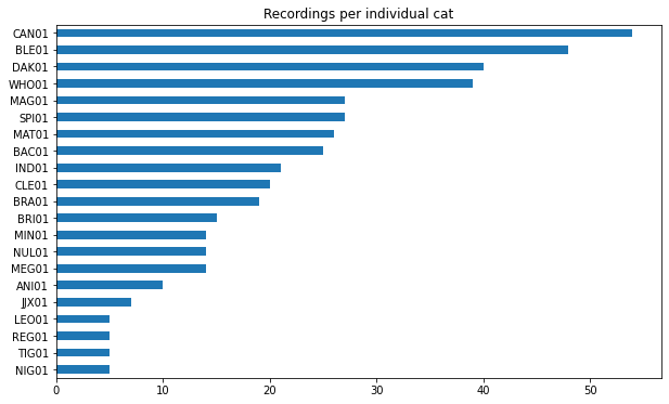
In fact, some cats occur way more often in the recordings than others. I don’t know why. Maybe “CAN01” is just very talkative whereas “NIG01” prefers to keep to himself? Number of recordings per individual cat:
Looking at these distributions is important. When we train a neural network to classify a given voice recording, we want to make sure it performs better than simply guessing the most frequent label.
For example, always guessing “female” when asked for the cat’s gender would be correct in 78% of cases because there are 345 female voice recordings and only 95 recordings of male cats.
Any classifier that is supposed to be useful has to surpass this baseline of “informed” guessing.
| Feature | Most frequent label | Absolute count | Relative count = baseline accuracy |
|---|---|---|---|
| Situation (3 classes) | isolation | 221 of 440 recordings | 50.2 % |
| Sex (2 classes) | female | 345 of 440 recordings | 78.4 % |
| Breed (2 classes) | european_shorthair | 225 of 440 recordings | 51.1 % |
Now we have an idea of what our data distributions look like. In total, there are three interesting tasks we can have a model learn from the data: (1) What situation was the cat in, (2) what is the sex of the cat, and (3) what is the breed of the cat. It will be interesting to see if these tasks can be learned from the data at all. Let’s start preparing our data to train a model.
Turning audio into images
There are many ways to encode an audio signal before passing it into a neural network. For my project, I am choosing a visual approach: We plot the spectrogram of the audio recordings as an image.
This allows us to use well-established neural networks from the field of computer vision. Also, spectrograms look nice.
Spectrograms are a plot where the location in the image represents a given frequency at a given point in time in the audio file. The brightness of a pixel represents the intensity of the audio signal.
The following example shows one of the recordings as a spectrogram. The time axis goes from top left (zero) to bottom left. The x-axis denotes the frequencies.
Image classification using a pretrained ResNet
Having turned our audio classification task into an image classification task, we can start with our model training. We are going to train three models for three different tasks:
- Given a spectrogram image, classify the situation the cat was in.
- Given a spectrogram image, classify the sex of the cat.
- Given a spectrogram image, classify the breed of the cat.
I have been playing around with the fast.ai library in the past few weeks which provides convenient wrappers around the PyTorch framework, so I decided to use fast.ai for this project.
Like most deep learning frameworks, it is easy to re-use popular computer vision architectures in fast.ai. With one(-ish) line of Python, you have a capable neural network for image classification at your hands. It comes pre-trained so that you need fewer images for your task at hand.
create_cnn_model(
    models.resnet18,
    n_classes,
    pretrained=True)
ResNets are a popular neural network architecture from 2015 that introduced residual connections - a mechanism that improves training behavior and allows the training of (very) deep networks.
The catmeows dataset is quite small, so I was satisfied with the smallest ResNet flavor (called ResNet-18). It has “only” 18 layers and it is still oversized for my 440 images.
The ResNet implementation wants to have square images as its input, so I took random square crops from the spectrograms during training. The crops were 81 x 81 pixels in size and could be from different points in time of the recording, but always contain the full spectrogram.
Figure: The pre-processed images as they go into the neural network. Here we are comparing recordings of female cats with male cats. Do you see a clear difference? I admit that I don’t.
Splitting the data for training and validation
When training a classifier it is important not to show all of your data to the model during training. You want to hold out some samples for validating the classifier during the training process. That way you get an idea if the model learns the training data by heart or if it actually learns something useful.
Sometimes it is fine to take a random percentage of the dataset as the validation set. In this case, I wanted to separate the cats across train and validation split so that the model can’t cheat by memorizing the characteristics of an individual cat.
I took 4 individual cats out of the training data. Their recordings combined made up 66 samples of the dataset, which means 15% of the data was reserved for validation and only the remaining 85% were used for training.
The results
For the three different tasks, the 3 models I trained achieved the following accuracy scores. For easy comparison, I also list the guessing baseline as described above.
| Task | Classification accuracy | Guessing baseline (see above) |
|---|---|---|
| Situation | 63.6 % | 50.2 % |
| Sex | 90.9 % | 78.4 % |
| Breed | 93.9 % | 51.1 % |
Results plot: Achieved model accuracy (blue) versus guessing baseline (grey).
Across all three tasks, the models performed well above the guessing baseline we have determined earlier.
Let’s also take a look at the confusion matrix for each task. A confusion matrix plots each sample of the validation set and indicates how many were classified correctly and which errors were made.
First confusion matrix that shows how well the classification of the situation worked. Some uncertainty shows: 10 samples are incorrectly classified as “waiting for food”, for example:
Second confusion matrix of the task to classify the sex of the cat in the recording. 60 out of 66 were classified correctly. Not bad, I think:
Third confusion matrix that shows how well the breed was classified. 62 out of 66 samples were classified correctly. I would not have expected this to work at all, to be honest.
What to make of this
First of all, these are quick results. We haven’t built a super AI that understands every single cat in the world. (Yet.)
What these results mostly show are interesting aspects of the dataset: Most of all, I was surprised how well the sex and breed can be told apart by the model. As I made sure to separate individual cats across train and validation data, I do have some confidence that the model didn’t cheat. There may still be some information leakage that I’m not aware of, of course.
What to improve
This is a small dataset. ResNet-18 is a big network. This mix can cause problems.
In my case, I am using a pre-trained version of ResNet, so the convolutional features don’t have to be learned from scratch. Still, I found myself re-running the training multiple times with varying success. I think with such little data it is still easy for the model to run into a local optimum and overfit on the training data.
Ideas for improvement:
Try freezing different layers and sets of layers of the network. It’s a tiny amount of data, we wouldn’t want to destroy the pre-trained features by accident. At the same time, spectrograms are not natural images, so fine-tuning probably makes sense.
Some additional data augmentation would surely help to enrich the training data. As these are not natural images but visualizations of an audio signal, I think some augmentation operations make sense (cropping at different points in time, jitter contrast, and brightness to simulate volume fluctuations). Some others are more questionable (perspective transformations, cropping different frequency bands). I haven’t tried them so far, but they could very well improve the results.
To learn more about the data, it would be interesting to extract quantitative audio characteristics and train a logistic regression or random forest on the data. These models are easier to interpret and could help to understand if the models look at something meaningful in the data or if there is some data leakage that allows the models to cheat.
Conclusion
Playing with public datasets is fun! You should try it.
I may continue with this pet project (pet! get it?) or start something fresh with the next dataset that looks interesting.
If you’ve found an issue in my data or training setup, please let me know.
You can find the complete project code in a messy Jupyter notebook on Github.
References
- The Datase to download: “CatMeows: A Publicly-Available Dataset of Cat Vocalizations” https://zenodo.org/record/4008297
- Paper that accompanies the dataset: https://air.unimi.it/handle/2434/811133
- ResNet, the original paper: https://arxiv.org/abs/1512.03385
Turns out I don’t need a neural network to let me know: Ginny is waiting for food.


